
Working with Tables in Excel
Content
- Introduction
- Special functionality of a Table
- Creating Your Table
- Table Options on the Ribbon
- Referencing cells in a table (structured referencing)
- Referring to a table from another workbook
- Other table advantages
- TableTools add-in
- Conclusion
- Links
Introduction
If you prefer watching video, here is a 45 recording of my "Modern Excel webinar" session of January 2020
A lot of the data you use in Excel is laid out as a table. Since Excel 2007 there is handy functionality for this called Format As Table. Contrary to what you might expect from this name however, the format bit is irrelevant or at best a nice side-effect.
This article introduces you into the concepts of working with Tables in Excel and shows you how they may help you in your everyday Excel use.
Special functionality of a Table
After defining a table, the area gains special functionalities:
1. Integrated autofilter and sort functionality
If your Table has a header row, it will always have filter and sorting dropdowns in place on the header row:
Sorting and filtering dropdowns
2. Easy selecting
Selecting an entire column or row is simple: move your mouse to the top of the table until the pointer changes to a down pointing arrow and click. The data area of that column is selected. Click again to include the header and total rows in the selection.

selecting an entire column of data within your table
You can also select the entire data area or the entire table by clicking near the table’s top-left corner (the mousepointer changes to a south-east pointing arrow):

Selecting all data within your table or the whole table is just
one or two clicks away.
3. Header row remains visible whilst scrolling
If your table is larger than fits on a screen and you scroll down, the column letters are temporarily replaced with the table’s column names (but only whilst you’re inside the table!):
Table header names on Excel’s column header when scrolling
4. Automatic expansion of table
If you type anything next to a table, Excel assumes you want to expand the table and automatically increases the table size to include your new entry. Of course you can undo this expansion too, or switch off this behavior entirely.
5. Automatic reformatting
When you insert or remove a row (or column) in your table, Excel will automatically adjust the formatting: alternate shading is kept nicely in place.
6. Automatic adjustment of charts and other objects source range
If you add rows to your table, any object that uses your table’s data will automatically include the new data.
Creating Your Table
Creating a table in Excel is easy. Of course you already have some data available somewhere on your sheet. Select the cells that contain the data:
Select the table area
Next, on the Home tab of the ribbon, find the group called "Styles". Click on the button that says "Format as Table":
"Format as Table" button on the Styles group of the Home tab.
After clicking this button, Excel shows a new user interface element called a gallery, with a number of formatting choices for your table:
Table format gallery.
Select one of the predetermined formats. After clicking one of the formats, Excel will ask you what range of cells you want to convert to a table. If your table contains a heading row, make sure the checkbox is checked. Click OK to convert the range to a table.
Dialog asking what range of cells has to be converted to a table.
After you’ve finished these steps, your table will look like this:
Range of cells, after converting to table
Table Options on the Ribbon
Once you have selected any of the cells within the table, you will see a new tab appear on the ribbon, called Table Tools, Design. Tis is what the ribbon will look like after you click this tab:
Ribbon after clicking the Table Tools tab.
Each group on this tab is discussed in the following paragraphs.
Properties group
The properties group enables you to do two things:
Properties group on Table Tools tab
1. change the Name of the table
The name of a table is used when you refer to cells within the table in a formula.
2. Change the size of the table
Click this control to change the size of your table.
Tools group
This group has three controls:
Tools group on Table Tools tab
1. Summarize with PivotTable
It is obvious what this control does. After you have created the pivot table, you don’t need to worry about updating the sourcerange of the pivot table anymore. If you add data to your table, Excel automatically expands the source range of the Pivot table to reflect your changes. Of course you still have to refresh the Pivot table to see the results.
2. Remove Duplicates
After clicking this control, you are presented with a dialog with which you can select the columns that you want to use to determine whether a row in the table is unique:
Remove Duplicates dialog
3. Convert to Range
By pressing this button you demote the table back to a normal range. Beware if you do this when you’ve based e.g. a pivot table on the range, the Pivot table’s source range will not be updated and the pivot table cannot be refreshed anymore.
The External Table Data Group
This group is all about the source data of a table and only applies if the data in the table has been imported into Excel using a database- or webquery or a sharepoint list.
External Table Data group on the Table Tools tab of the ribbon
This group has 5 buttons:
1. Export Data
This is in fact a combobutton. If you press it you’re offered two options,
"Export Table to SharePoint List" and "Export Table to Visio PivotDiagram". What these are exactly is beyond the scope of this article.
2. Refresh
Use this combobutton to refresh the external data in your table. If you click the arrow beneath the button, you’re offered a menu which amongst others also includes "Refresh All", with which you can refresh all external data ranges in your file.
3. Data Range Properties
This button can be used to change the properties of the external data you have based your table on.
4. Open in Browser
If your table is a sharepoint list, this button enables you to open a browser window with that list.
5. Unlink
If your table is a sharepoint list, this button disconnects the table from the list.
Table Style Options Group
This group houses the controls which determine how table styles are applied to your table:
Table Style Options group on the Table Tools tab of the ribbon
1. Header Row
When this box is unchecked, Excel removes the header row from your table. The cells of the header row are cleared, but Excel does remember the header. If you type anything into any cell in that now empty row, Excel will not overwrite that information when you check the box again. Instead, Excel will insert a new row to show the header. Cells below the table are then moved down.
2. Total Row
Check this box if you want a total row below your table. Excel will automatically add a sum function below the last column in your table.
3. Banded Rows
Check this box to get alternating shading for the rows in your table.
4. First Column
If you check this box, the first column of your table will be formatted differently from the other columns.
5. Last Column
Formats the last column of your table differently from the other columns.
6. Banded Columns
Check this box to get alternating shading for the columns in your table
Table Styles Group
The last group on the Table Tools tab enables you to quickly change the style of your table:
Table Styles group on the Table Tools tab of the ribbon
Click the dropdown button to the right of the gallery to see all choices available to you. Hover over a particular style to see what your table would look like when you click it. At the bottom of the gallery there are two extra choices:
1. New Table Style
This option enables you to create your own table style.
2. Clear
Use this to remove the table style from your table entirely. Number formats are retained.
Referencing cells in a table (structured referencing)
To refer to cells inside a table, a special syntax can be used called "Structured References". To see how this works, click in a cell to the immediate right of the table, hit the = sign, type SUM( and then click on any cell with data within the table. You’ll get a formula like this one:
=SUM(Table3[@Discount])
The naming convention to refer to the cells in your table works as follows:
Table3: The name of your table
@: Denotes the data comes from the same row your formula cell is in
Discount: The name of the column in the table
Some other examples:
Because of this naming convention, you are not allowed to have more than one column inside a table with a specific heading. As soon as you try to type a new heading that duplicates an existing one, Excel will automatically correct the duplication by appending a number to the new column name.
A nice feature of tables is immediately shown as soon as you hit enter: your table is automatically resized to include your formula (Excel has also made up a column heading for you) and the formula is automatically copied down to fill the entire column alongside your data! Both actions may be undone by using the smart tag that appears.
Referring to a table from another workbook
Even though I mentioned that a table is also stored as a range name there is a peculiarity. The range name points only to the data rows of the table. The header row is NOT included. This means that if you want to create a pivot table on data that is in a table in another workbook you need to use a syntax that differs from the old days.
Normally you would refer to a range name "TableName" in workbook "WorkbookName.xls"
using: [WorkbookName.xls]!TableName
But although a table is represented by a range name, you should not use
the range name syntax as the source. Rather you must use this:
WorkbookName!TableName
This will convince Excel that you are pointing to a table and then includes the header rows.
Other table advantages
Using a table is advantageous on Excel for Android as well. It will enable you to edit records in the table by going into Card view, which makes it a LOT easier to work with the records in the table:
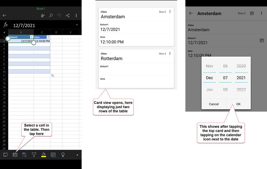
Table Tools add-in
Together with fellow Excel MVP Frederic Le Guen I devised a small add-in to make your table life a little simpler.
The tool adds a tab to the ribbon called Table Tools:

And a right-click menu which differs whether you right-click within a table or outside of a table:
- Within a table it shows the columns names so you can quickly goto
a column
- Outside of a table it shows a list of tables in the active workbook
- If you use the Table Name editbox on the TableTools ribbon tab, it will not only rename the table, but also automatically update all queries which use this table with the new name
- If you edit a column name in a table, the tool will update all PowerQuery queries with this new name.
- Note that the tool has an improved interface to convert a range
to a table, which enables you to name the table right when you define
the table
- In addition, you can add a comment to the table right there, which
appears when you type a formula:
Conclusion
As you have seen, Tables are a great addition to Excel’s features. Most of these features were already part of Excel 2003's List feature. But Excel versions 2007 and up builds upon that feature, significantly improving it. The most important benefits are:
- Integrated autofilter and sort functionality
- Easy selecting
- Header row remains visible whilst scrolling
- Automatic expansion of table
- Automatic reformatting
- Automatic adjustment of charts and other objects source range
Links
If you're interested in VBA, read about Excel Tables and VBA here.
Ron de Bruin has written a nice add-in to ease working with tables.
Frequently asked Questions
What is the purpose of using Tables in Excel?
What special functionalities does an Excel Table provide?
How do you create a Table in Excel?
What options are available on the Table Tools ribbon tab?
How do you reference cells inside an Excel Table using structured referencing?
How can you refer to a Table from another workbook?
What are some advantages of using Tables on Excel for Android?
What is the TableTools add-in and what features does it provide?
What are the main benefits of using Tables in Excel?
Where can I find additional resources or add-ins related to Excel Tables?
Comments