
Batchprocessing: how to calculate your model with many input values
An article by Niek Otten, Excel MVP.
Introduction
Sometimes you want to apply an existing worksheet calculation to many sets of data rather than just the one case for which it was designed. For example, you developed a worksheet which calculates your pension. It accepts some twenty input variables and generates five output variables.
Then your boss demands that you apply that one-time worksheet to 500 employees.
Of course you could write some VBA code to do this. But many people hesitate to use VBA and often they are not even allowed to, on their work PC. Fortunately, there is a solution that does not require VBA. Excel has a feature for doing this, the Data, Table command. But it's not well documented.
Each time I was asked to do something complex using a Data Table, it took me a while to remember how to do it. So I developed this recipe. It may seem like a lot of steps, but it's actually very straightforward and can be done in minutes.
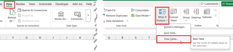
Where do I find this feature
Click the Data tab. On the right you should find the What-if Analysis drop-down button. Click it and you'll seet Data Table as the third option:
Step 1.
Make a copy of your original workbook, and use that to work with in the following steps. (Always make a backup before attempting anything big or new.)
Step 2.
Just an informational step. So that you can keep things clear, we will be dealing with three pages, called:
Source WS (worksheet):
The big table of input data you want to work with, such as the 500 employees' data. Aside from making it row oriented in the next step, this will not be edited/affected in any way.
Model WS:
Your existing worksheet which calculates one set of inputs at a time. This will only have its input cells changed, in Step 6.
Data Table WS:
A new worksheet with the Data Table, including its results. This is where almost all your editing will be done.
Step 3.
Import your source data into an Excel worksheet (of course). This is the "Source WS". All the data (input variables) for each Source WS record must be on one row (line). So work your data into a one-row format, if it covers multiple rows per input situation. If you have extra columns of data, they don't matter; just leave them. All that's needed is that each row of input data has all its data on one row. Input columns do not have to be next to each other.
Step 4.
Now on to the good stuff. In your Source WS, define Names (Insert /Name /Define) for the columns you need as input. If the columns have a header, do not include the header in the name. So the first line of the named area should be the first line of your variable data.
You can save yourself some time by having Excel define the names for you by using the button "Create From Selection" in the Defined Names group on the Formulas tab of the ribbon. Make sure you only select the "Top row" check box.
Step 5.
Insert a new sheet into your workbook. This is your "Data Table WS". Across row 1, starting in column B, fill the column headers (text) with the input column headers as defined in step 4. In cell A2, enter the number 1. In cell B2, enter the formula =INDEX(SourceColumn,A2), where SourceColumn is just an example of a Named range you created in step 4. Each input variable should get a similar formula in its own column.
Step 6.
On your Model WS, make all your Model's input cells refer to the input columns of row 2 of the Data Table WS. So the first Model input field now has "=DataTable!B2" as a formula, instead of an input value, the second one "=DataTable!C2", etc. Do this for all the input fields in the Model.
Step 7.
Extend your Data Table WS to receive output by making new column headers in Row 1, to the right of the input columns. (Actually, they don't have to be to the right, as long as you keep things straight.).
Now make the output fields in row 2 of the Data Table WS refer to the output fields of the Model WS. Just simple references like "=Model!C37" or "=Sheet17!C37".
Step 8.
Test it. Enter an index number in A2 and check that it retrieves the correct input from the Source WS and generates the correct output, all on this one line.
Step 9.
Starting in cell A2, fill down a series of consecutive numbers (1,2,3...), for however many Source records you have. Don’t use a formula for this; use the fill handle, the Edit>Fill>Series command, fill it in by hand, use a +1 formula and convert using Copy/Paste Special/Values - anything that will make it a "hard" number, NOT a formula.
Step 10.
On the Data Table WS, select cells A2 to the last line and the last column of the table and then choose Data, Table from the menu or click the Data Table button on your Quick Access Toolbar. In the dialog box, leave "Row input cell" blank. In the "Column input cell" box, enter A2. Click OK, and see your table filled with input data and computed results. Voila!
How long did it all take... 7 minutes?
Frequently asked Questions
What is batch processing in Excel and why would you use it?
Where can I find the Data Table feature in Excel?
Why should I make a copy of my workbook before starting batch processing?
What are the three worksheets involved in this batch processing method?
How should I organize my source data for batch processing?
How do I define names for input columns in my source worksheet?
How do I link my model worksheet input cells to the data table worksheet?
What is the correct way to fill the index numbers for the data table?
How do I create the data table to calculate results for multiple input sets?
How can I test if the data table setup is working correctly?
Comments